Getting started with R

Main Page

Installation
A few commands
Data and objects
Accessing the values of an object
Operators
A few functions

Installation

First of all:

Install R from the web site Rproject. R is a open-source (i.e. free) software.
Install Rstudio from the web site RStudio. RStudio allows the user to run R in a more user-friendly environment. It is a open-source (i.e. free) software.

RStudio screen is divided in several windows.

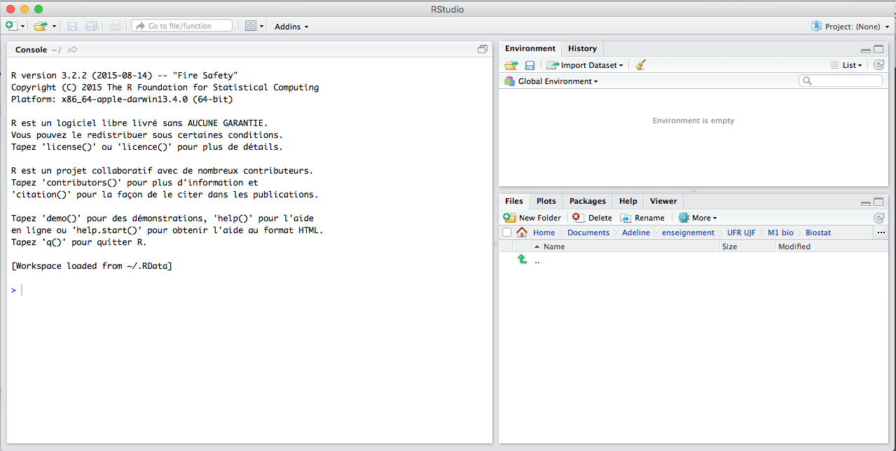
Alt text

The console (lower left corner) is where you can type the commands and see output. Run the commands with Enter.
The script (upper left corner) is where you can write the 'script' to save all your commands. Run them down to the lower left corner by Ctrl+R (Windows) or Cmd+Enter (Mac).
The workspace (upper right corner) tab shows all the active objects. The workspace tab stores any object, value, function or anything you create during your R session. The {} tab shows a list of commands used so far. The history tab keeps a record of all previous commands.
The files (lower right corner) tab show all the files and folders in your default workspace as if you were on a PC/Mac window. The plots tab will list a series of packages or add-ons needed to run certain processes. For additional info, see the help tab.

If you have different projects, we recommend to create a folder for each project. Then you can change the R working directory using the function setwd:

R>    getwd() # Shows the working directory (wd)
R>    setwd("/M1 bio/Biostat") # Changes the wd

A few commands

An object can be created with the "assign" operator which is written as an arrow with a bracket and a minus sign.

R>  n <- 10

One of the simplest commands is to type the name of an object to display its content.

R> n
[1] 10

The digit 1 within brackets indicates that the display starts at the first element of n.

R is case sensitive (lower case different from capital letters).

R> x <-1
R> X <-10
R> x
[1] 1
R> X
[1] 10

Note that you can type an expression without assigning its value to an object, the result is displayed on the console but not stored in memory:

R> (10 + 2) * 5
[1] 60

The function ls lists the objects in memory.

R> ls()
 [1] "A"             "D"             "D1"            "Dyndoc.Vec"   
 [5] "dynRbVar"      "dynVar"        "dynVarWithArg" "E"            
 [9] "Fo"            "freq"          "G1"            "G2"           
[13] "Hy"            "HY"            "LenzI"         "LenzT"        
[17] "M"             "ms"            "mu"            "muC"          
[21] "muR"           "n"             "N"             "p"            
[25] "pstatus"       "pstatusadB"    "pstatusadBH"   "pstatusadBY"  
[29] "q"             "R"             "R2"            "S"            
[33] "sample"        "sdC"           "sdf"           "sdR"          
[37] "sds"           "sig"           "SS"            "Tmu1"         
[41] "TRS"           "x"             "X"             "Y"

The on-line help of R gives useful information on how to use the function. Help is available directly for a given function. For example:

R> ? hist

displays the help page for the function hist() (histogram).

Data and objects

Objects

Objects in R are characterized by two attributes which specify the kind of data represented by an object. In order to understand the usefulness of these attributes, consider a variable that takes the value 1, 2, or 3: such a variable could be an integer variable (for instance, the number of eggs in a nest), or the coding of a categorical variable (for instance, grade of cancer).

It is clear that the statistical analysis of this variable will not be the same in both cases: with R, the attributes of the object give the necessary information.

All objects have two attributes: mode and length. The mode is the basic type of the elements of the object; there are four main modes: numeric, character, complex, and logical (FALSE or TRUE). The length is the number of elements of the object. To display the mode and the length of an object, one can use the functions mode and length, respectively:

R> x<-1
R> mode(x)
[1] "numeric"
R> length(x)
[1] 1

Whatever the mode, missing data are represented by NA (not available).

Reading data in a file

For reading and writing in files, R uses the working directory. To find this directory, the command getwd() (get working directory) can be used, and the working directory can be changed with setwd("C:/data"). It is necessary to give the path to a file if it is not in the working directory.

Data can be read with the function read.table or scan. The function read.table creates a data frame. For instance, a file named datafile.csv can be read:

R> mydata <- read.table("data/datafile.csv")

In that command, mydata is the name you choose for the data frame. By defaults, each variable of the data frame is named V1, V2, .... They can be accessed individually by mydata$V1, mydata$V2, ... or by mydata["V1"], mydata["V2"], ... or by mydata[, 1], mydata[, 2], ....

All the options of the function read.table are described in the help file. For example, if the file contains the names of the variables on its first line, we can use the option header, if the cells are separated by ; , we can use the option sep=";":

R> XY <- read.table("data/datafile.csv",header=TRUE,sep=";")

Example To upload the data set called hypoxy.csv, run the following instruction:

R> HY <- read.table("data/hypoxy.csv", header=TRUE, dec=",")

To check if the data were correctly loaded, use the function head that displays the first 6 rows of the dataset:

R> head(HY)
   Level Name_Prot Hypoxy Training N_Rat Location
1 0.9843      RyR2     No       No    N1       TA
2 0.9419      RyR2     No       No    N2       TA
3 0.7761      RyR2     No       No    N5       TA
4 0.8668      RyR2     No       No    N7       TA
5 1.2249      RyR2     No       No    N9       TA
6 1.2061      RyR2     No       No   N10       TA

All the values of the first six rows are displayed, the first is numeric, the five others are not.

Generating data

a:b creates a vector of values from a to b.

Example: to create the vector (1,2,3,4,5), use the command

R> 1:5
[1] 1 2 3 4 5

The resulting vector has 5 elements. Arithmetic operators can be used:

R> 1:5-1
[1] 0 1 2 3 4
R> 1:(5-1)
[1] 1 2 3 4

seq(a, b, step) generates a sequence of real numbers starting from a ending at b with increment step.

Example: create a vector with 9 equispaced numbers between 1 and 5:

R> seq(1, 5, 0.5)
[1] 1.0 1.5 2.0 2.5 3.0 3.5 4.0 4.5 5.0

c(X,Y) concatenates two or more vectors or values in a row to make a new vector.

Example: add a value 6 to the vector X equal to (1,2,3,4,5):

R> X <- 1:5
R> c(X,6)
[1] 1 2 3 4 5 6

rep(a, n) creates a vector with all its elements identical.

Example: create a vector with 10 elements equal to 1:

R> rep(1, 10)
 [1] 1 1 1 1 1 1 1 1 1 1

gl(k, n) generates regular series of factor: k is the number of levels (or classes) and n is the number of replications in each level.

Example: create a vector with 1 repeated 5 times, 2 repeated 5 times and 3 repeated 5 times:

R> gl(3, 5)
 [1] 1 1 1 1 1 2 2 2 2 2 3 3 3 3 3
Levels: 1 2 3

cbind(X,Y) binds two or more vectors with same length, as columns.

Example: Create first the vector Y <- c(1,4,9, 16, 25). Check the length of Y and bind the two vectors X and Y:

R> Y <- c(1,4,9, 16, 25)
R> cbind(X,Y)
     X  Y
[1,] 1  1
[2,] 2  4
[3,] 3  9
[4,] 4 16
[5,] 5 25

rbind(X,Y) binds two or more vectors with same length, as rows.

Example: Bind the two vectors X and Y in row:

R> rbind(X,Y)
  [,1] [,2] [,3] [,4] [,5]
X    1    2    3    4    5
Y    1    4    9   16   25

matrix(vec, nrow) creates a matrix with values of vector vec with nrow rows.

Example: Create a matrix with elements from 1 to 6, with 2 rows and 3 columns:

R> A <- matrix(1:6,2)
R> A
     [,1] [,2] [,3]
[1,]    1    3    5
[2,]    2    4    6

dim(XY) number of rows and columns of a matrix XY.

Example:

R> XY <- cbind(1:10,11:20)
R> dim(XY)
[1] 10  2

Accessing the values of an object

X[ind] extracts from vector X, coordinates specified by ind. The entry ind may be:

a vector of integers specifying the indices to be selected,
a vector of Booleans (the TRUE coordinates will be selected),
a vector of names to be selected (if X has names).

Example: display the third element of X and Y:

XY[row,col] extracts from matrix or data frame XY, cells corresponding to particular rows and columns. The entries row and col may be:

empty (understood as “all” rows or columns),
a vector of integers specifying the indices to be selected,
a vector of Booleans (the TRUE coordinates will be selected),
a vector of row or column names to be selected.

Example:

head(XY) first 6 rows of matrix or data frame XY.

Example:

R> head(XY)
     [,1] [,2]
[1,]    1   11
[2,]    2   12
[3,]    3   13
[4,]    4   14
[5,]    5   15
[6,]    6   16

A$a Accessing the values of an object A with names.

Example:

R> colnames(A) <- c("a", "b", "c")
R>  A
     a b c
[1,] 1 3 5
[2,] 2 4 6
R>  A<-as.data.frame(A)
R>  A$a
[1] 1 2

Operators

Arithmetic operators

+ addition
- subtraction
* multiplication
/ division
^ power

R> 2^2
[1] 4

Comparison operators

< lesser than
> greater than
<= lesser than or equal to
>= greater than or equal to
== equal
!= different

Example

R> x <- 0.5
R> (0 < x)
[1] TRUE
R> x <- 1:3
R> y <- 1:3
R> (x == y)
[1] TRUE TRUE TRUE

Logical operators

!x logical NOT
x & y logical AND
x && y id.
x | y logical OR
x || y id.

Example:

R> x<-1:6
R> y<-4:9
R> (x>5)
[1] FALSE FALSE FALSE FALSE FALSE  TRUE
R> ! (x>5)
[1]  TRUE  TRUE  TRUE  TRUE  TRUE FALSE
R> (x<3)&(y>4)
[1] FALSE  TRUE FALSE FALSE FALSE FALSE
R> (x<5)&(y>4)
[1] FALSE  TRUE  TRUE  TRUE FALSE FALSE

A few functions

sum(X) adds all values in vector X. If X is Boolean (TRUE/FALSE), the number of TRUE’s is returned.

Example:

R> sum(X)
[1] 15

cumsum(X) returns the vector of cumulative sums for the values in X: first, first plus second, first plus second plus third, etc.

Example:

R> cumsum(X)
[1]  1  3  6 10 15

rowSums(XY), colSums(XY) sums in each row, in each column of a matrix XY.

Example:

R> rowSums(XY)
 [1] 12 14 16 18 20 22 24 26 28 30
R> colSums(XY)
[1]  55 155