Probabilities

Probabilities

Main Page

Random experiments

Introduction to randomness

A random experiment may have different outcomes when repeated. Let us give some definitions. The two main rules to compute the probability of an event are: In R, values of a random experiment can be obtained by simulation. The first function to simulate the realisation of a random experiment is the sample function. Example Let us define the vector x=(0,1).

R> x<-c(0,1)

sample draws a random permutation of x.

R> sample(x)
[1] 0 1
R> sample(x)
[1] 1 0

Try to repeat 10 times. How many times did you get each of the two permutations?

Let us now sample 100 random values from x, repetitions allowed:

R> A <- sample(x,100,replace=TRUE)             # random sample

table(A) gives the number of 0 and 1 obtained in A. The sum of the two absolute frequencies is equal to 100, the number of random values that have been drawn.

R> table(A)
A
 0  1 
44 56

If you run again the instruction sample, you will obtain different absolute frequencies.

R> A <- sample(x,100,replace=TRUE)             # random sample
R> table(A)
A
 0  1 
53 47

Example We can also draw values from a qualitative variable. Set x=(a,b,c).

R> x<-c("a", "b", "c")

A random permutation of x is obtained with

R> sample(x)
[1] "a" "c" "b"

A random subset of x is obtained with

R> sample(x,2)
[1] "b" "c"

We can also draw values of x with possible repetitions, as before:

R> A <- sample(x,100,replace=TRUE)
R> table(A)
A
 a  b  c 
35 28 37

Random variables

Example

Random variables are categorized in two families, discrete and continuous.

Probability distributions

In this section, we define the main characteristics of a random variable. These notions are illustrated below for each distribution. The notions below depend on the random variables only through their probability distributions. They are called theoretical, as opposed to empirical when evaluated over a statistical sample.

In what follows X and Y denote numeric random variables.

Theoretical mean

Let us start with the most intuitive characteristic: the mean.

The following rules apply for the mean:

• The mean of the sum of two random variables is the sum of their means:
  𝔼(X + Y)=𝔼(X)+𝔼(Y)
  

• The mean of a rescaled variable is the rescaled mean:
  𝔼(aX)=a𝔼(X)
  

• The mean of the product of two independent variables X and Y is the product of their means:
  𝔼(XY)=𝔼(X)×𝔼(Y)
  

Theoretical variance

The following rules apply for the variance:

The theoretical standard deviation is the square root of the variance.

Cumulative distribution function

The cumulative distribution function (cdf) maps a value x onto the probability to be less or equal to the value: F(x)=Prob(X ≤ x).

Quantile function

The quantile function is the inverse of the cumulative distribution function. It maps a probability u onto the value x such that u = F(x).

Discrete distributions

Note that its mean is 𝔼(X)  =  ∑ x_i p_i.

Classical discrete distributions are Bernoulli, binomial, Geometric, Hypergeometric. We detail below the two first ones.

Bernoulli distribution

Simulation from the Bernoulli distribution Example

R> p<-0.5
R> rbinom(1,1,p)
[1] 1
R> rbinom(10,1,p)
 [1] 0 0 1 1 1 0 0 0 1 0

The empirical proportion of 1 changes with the sample, but is close to the theoretical proportion p when the size of the sample is high:

R> prop.table(table(rbinom(100,1,p)))

   0    1 
0.55 0.45 
R> prop.table(table(rbinom(1000,1,p)))

    0     1 
0.517 0.483 
R> prop.table(table(rbinom(10000,1,p)))

     0      1 
0.5015 0.4985

R computes the probability, cumulative distribution, and quantile functions for standard families of probability distributions.

Example The probability of success (value 1) of a Bernoulli distribution with parameter p=0.2is

R> dbinom(1,1,0.2)
[1] 0.2

The probability of failure is

R> dbinom(0,1,0.2)
[1] 0.8

Binomial distribution

Example From past experience, it is known that a certain surgery has a 90% chance to succeed. This surgery is going to be performed on 5 patients. Let X be the random variable equal to the number of successes out of the 5 attempts. X follows a binomial distribution with parameters n = 5 and p = 0.9.

Simulation from the binomial distribution Example Simulate one value of the binomial distribution with parameters 5 and 0.9.

R> n<-5
R> p<-0.9
R> x<-rbinom(1,n,p)
R> x
[1] 5

We can also compute the probability to have 0 success, exactly 1 success (among the 5 surgeries), 2 succcesses, etc. These theoretical probabilities are computed with the function pbinom.

Example Apply functions dbinom, pbinom, qbinom for the surgery example.

R> dbinom(4,n,p)
[1] 0.32805

R> dbinom(2,n,p)
[1] 0.0081

Cumulative probabilities are the probabilities to obtain at most a certain value, or at least a certain value. They are calculated with pbinom, using the option lower.tail=FALSE for the condition at least.

R> pbinom(4,n,p)
[1] 0.40951

R> pbinom(3,n,p, lower.tail=FALSE)
[1] 0.91854

The (theoretical) cumulative distribution has to be compared to the empirical cumulative distribution function (ecdf) of a binomial sample.

Code R :

R> X<-rbinom(1000,n,p)
R> plot(ecdf(X))
R> curve(pbinom(x,n,p), col='red', add=TRUE)

Résultat :

Continuous distributions

Uniform distribution

Example Simulating from the uniform distribution on the interval [0, 5] is performed with the function runif:

R> runif(1,0,5)
[1] 1.803786

Normal distribution

The normal or Gaussian distribution 𝒩(μ, σ) has mean μ, standard deviation σ.

Example Simulate 1000 values of the normal distribution with parameters μ = 1 and σ = 10.

R> mu<-1
R> sig<-10
R> x<-rnorm(1000, mu, sig)
R> mean(x)
[1] 1.145378

Code R :

R> hist(x)

Résultat :

The theoretical density is close to the histogram represented in the relative frequencies scale. Code R :

R> hist(x, prob=TRUE)
R> curve(dnorm(x, mu, sig), -40, 30, col="red", add=TRUE)

Résultat :

The (theoretical) cumulative distribution has to be compared to the empirical cumulative distribution function (ecdf) of a binomial sample. Code R :

R> X<-rnorm(1000,mu,sig)
R> plot(ecdf(X))
R> curve(pnorm(x,mu,sig), col='red', add=TRUE)

Résultat :

Let us continue with some properties of the normal distribution. The family of normal distributions is invariant through linear combinations of independent variables.

The function qqnorm draws the empirical quantiles of a sample against the quantiles of the standard normal distribution.

Example Let us simulate a sample X from the normal distribution 𝒩(0, 1) and draw its qqplot. Code R :

R> X<-rnorm(1000)
R> qqnorm(X)
R> abline(0,1)

Résultat :

Due to invariance through scaling, if the sample is drawn from the normal distribution 𝒩(μ, σ), the plot is close to the straight line with intercept μ and slope σ. Code R :

R> mu<-5
R> sig<-3
R> X<-rnorm(1000, mu, sig)
R> qqnorm(X)
R> abline(mu,sig)

Résultat :

Example The total nutritional intake (in Kcal per day) in the control population has mean 2970 and standard deviation 251. Among runners, the mean is 3350 and the standard deviation 223.

Consider a person taken at random in the control population. Would you say that the chances that the intake is smaller than 3000 are larger than 1/2?

R> muC<-2970
R> sdC<-251
R> pnorm(3000, muC,sdC)
[1] 0.5475691

What proportion of intakes in the control population are smaller than 2600?

R> pnorm(2600, muC,sdC)
[1] 0.07022685

What proportion of intakes in the runners population are smaller than 2600?

R> muR<-3350
R> sdR<-223
R> pnorm(3000, muR,sdR)
[1] 0.05826496

Which lower bound is such that 1% of the control population is below?

R> qnorm(0.01, muC,sdC)
[1] 2386.087

Which upper bound is such that 1% of runners are above?

R> qnorm(0.01, muR,sdR,lower.tail=FALSE)
[1] 3868.776

We continue the presentation of continuous distributions with two families, Student and Chi-squared, that are linked to the Gaussian distribution.

Student distribution

The Student distribution is defined from a Gaussian sample X₁, …, X_n, that is from n variables that are independent and identically distributed from a Gaussian distribution 𝒩(μ, σ). Let us denote $\overline{X}$ the empirical mean of the sample, and S² its empirical variance. The Student distribution is defined as follows:

The Student distribution is used for theoretical mathematical study of statistical notions such than confidence intervals, statistical tests.

The R functions associated to the Student distribution are named:

Example Simulate a sample from a Student distribution with 10 degrees of freedom (using the function rt) and represent its distribution: Code R :

R> X<-rt(1000, df=5)
R> hist(X, prob=TRUE, xlim=c(-5,5), breaks=30)

Résultat :

Let us try to compare both distributions, the empirical distribution is the histogram, the theoretical density of the Student distribution is in red, and the theoretical density of a standard normal distribution is in blue. Code R :

R> X<-rt(1000, df=5)
R> hist(X, prob=TRUE, xlim=c(-5,5), breaks=30)
R> curve(dt(x,df=5), col="red", add=TRUE)
R> curve(dnorm(x), col="blue", add=TRUE)

Résultat :

When the degree of freedom increases, the difference with the normal distribution decreases: Code R :

R> X<-rt(1000, df=100)
R> hist(X, prob=TRUE, xlim=c(-5,5), breaks=30)
R> curve(dt(x, df=100), col="red", add=TRUE)
R> curve(dnorm(x), col="blue", add=TRUE)

Résultat :

The difference between the Student and the Gaussian distributions can also been viewed via the qqnorm representations. Code R :

R> X<-rt(1000, df=5)
R> qqnorm(X)
R> abline(0,1)

Résultat :

Increasing the degree of freedom yields to a qqnorm close to a straight line. Code R :

R> X<-rt(1000, df=100)
R> qqnorm(X)
R> abline(0,1)

Résultat :

Chi-squared distribution

The Student distribution is defined from a Gaussian sample X₁, …, X_n, that is from n variables that are independent and identically distributed from a Gaussian distribution 𝒩(μ, σ). Let us denote $\overline{X}$ the empirical mean of the sample, and S² its empirical variance. The Student distribution is defined as follows:

The Chi-squared distribution is used for theoretical mathematical study of statistical notions such than confidence intervals, statistical tests.

The R functions associated to the Chi-squared distribution are named:

Example Simulate a sample from a Chi-squared distribution with 10 degrees of freedom (using the function rchisq) and represent its distribution: Code R :

R> X<-rchisq(1000, df=5)
R> hist(X, prob=TRUE)
R> curve(dchisq(x, df=5), add=TRUE, col="red")

Résultat :

Increasing the degree of freedom translates the distribution: Code R :

R> X<-rchisq(1000, df=10)
R> hist(X, prob=TRUE)
R> curve(dchisq(x, df=10), add=TRUE, col="red")

Résultat :

Fluctuation interval

A fluctuation interval with level q is such that the probability of values inside is q. It can be:

• Two-sided: (x₁, x₂). The probability to be below x₁ and the probability to be above x₂ are both equal to (1 − q)/2.
• Left-sided: (min, x₁). The probability to be below x₁ is q. The left bound min is the minimal value of the distribution (it can be −∞).
• Right-sided: (x₂, max) The probability to be above x₁ is q. The right bound max is the maximal value of the distribution (it can be +∞).

Fluctuation interval for the normal distribution

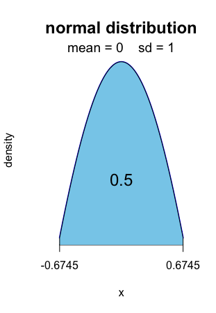
The normal.fluctuation function has been developed to illustrate and understand the fluctuation interval for a normal distribution. It takes a probability, the parameters of the normal distribution and the alternative (two-sided, less, greater). It returns the two quantiles that define the fluctuation interval.

The two-sided fluctuation interval with level 0.5 of the standard normal distribution is computed [ − 0.6745, 0.6745].

R> normal.fluctuation(0.5, mean=0, sd=1)

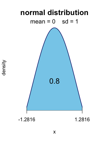
For level 0.8, it is [ − 1.2816, 1.2816].

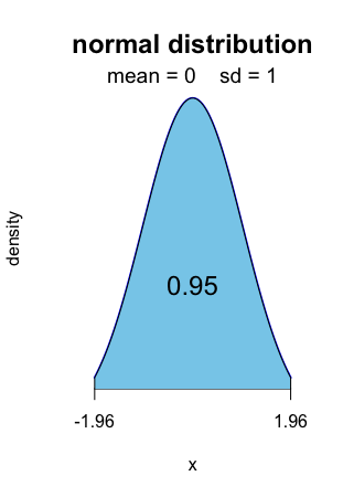
For level 0.95, it is the well-known [ − 1.96, 1.96].

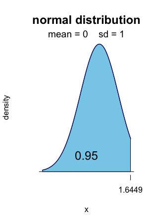
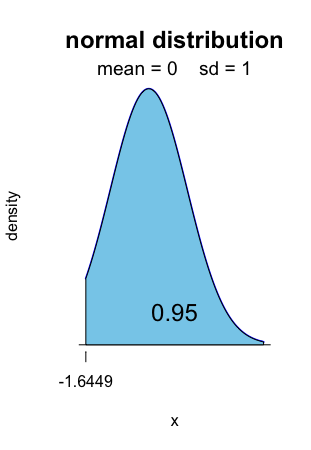
The left-sided fluctuation interval with level 0.95 is ] − ∞, 1.6449].

The right-sided fluctuation interval with level 0.95 is [1.6449, +∞[.

Limit theorems

Statistics are based on two powerful limit theorems, called the law of large numbers and the central limit theorem.

Law of large numbers

Example Define x = (0, 1) and for n=1000, we simulate a sample of n random values from x.

R> x<-c(0,1)
R> n<-1000
R> A<-sample(x,n,replace=TRUE)

Then, we compute the vector of cumulative sums of A, divide it by 1:n to compute the consecutive means of A.

R> M<-cumsum(A)/1:n

Then we plot M against 1:n as blue dots. The law of large numbers says that these empirical means (M) converge to the theoretical mean, which is equal to 0.5. Code R :

R> plot(1:n,M, col="blue", pch='.')
R> abline(h=0.5,col="red")

Résultat :

Central limit theorem

The Central Limit Theorem says that, if a large number of independent random variables having the same distribution are added, their sum approximately follows a normal distribution.

Normal approximations

As a consequence of the central limit theorem, some distributions can be approximated by the normal distribution with same mean and standard deviation.

• The binomial distribution ℬ(n, p) is close to the normal distribution $\mathcal{N}\left(np,\sqrt{np(1-p)}\right)$, for n large.

• The Student distribution 𝒯(n) is close to the normal distribution 𝒩(0, 1), for n large.

• The chi-squared distribution 𝒳²(n) is close to the normal distribution $\mathcal{N}\left(n,\sqrt{2n}\right)$, for n large.

• For a large sample from any distribution with mean μ, standard deviation σ, the z-scores $\displaystyle{\sqrt{n}\,\frac{\overline{X}-\mu}{\sigma}}$ and $\displaystyle{\sqrt{n}\,\frac{\overline{X}-\mu}{\sqrt{S^2}}}$ approximately follow the 𝒩(0, 1).

Example From past experience, it is known that a certain surgery has a 90% chance to succeed. This surgery is performed by a certain clinic 400 times each year. Let N be the number of successes next year.

The exact model for N is a binomial distribution with parameters n = 400 and p = 0.9 ($(n,p)). The normal approximation is 𝒩(360, 6). The two densities are represented (blue for the binomial density, red for the normal density): Code R :

R> n<-400
R> p<-0.9
R> curve(dnorm(x,mean=n*p, sd=sqrt(n*p*(1-p))), from=320, to=n, col="red", ylab="")
R> points(dbinom(0:n,n,p), col="blue")

Résultat :

Let us compute the probabilities for the clinic to perform successfully the surgery at least 345 times, in the exact and approximate models.

R> n<-400
R> p<-0.9
R> ms<-n*p
R> sds<-sqrt(n*p*(1-p))
R> pbinom(344,n,p,lower.tail=FALSE)            # exact model
[1] 0.9933626
R> pnorm(344,ms,sds,lower.tail=FALSE)          # approximate model
[1] 0.9961696

The insurance accepts to cover a certain number of failed surgeries; that number has only a 1% chance to be exceeded. Let us compute this number, in the exact and approximate models?

R> n-qbinom(0.01,n,p)                          # exact model
[1] 55
R> n-qnorm(0.01,ms,sds)                        # approximate model
[1] 53.95809